Blog — Page 4

Version 3.9.0 Release Notes

by Pavel Holoborodko on November 20, 2015

Over the course of the last three months we have added many important improvements and bug fixes into toolbox. We decided to produce the new official release as it contains critical updates for all platforms (even though eigensolver for large sparse matrices is not included yet).

Here is the main changes:

The Core: Multithreading manager has been updated with better load-balancing and non-blocking synchronization. This results in 15-20% performance boost in all operations with dense matrices, even including the matrix multiplication.
Eigenvalues.
- Speed of unsymmetric generalized eigen-decomposition has been improved. Now toolbox uses blocked version of Hessenberg tridiagonal reduction^[1] which gives us timings lower by 20%.
- Speed of symmetric eigen-decomposition has been boosted up as well. All cases are covered, including the standard and generalized problems in quadruple and arbitrary precision modes and both complexities.
  Actual speed-up factor depends on number of cores and matrix size. In our environment Core i7/R2015a/Win7 x64 we see x3 times ratio for 1Kx1K matrix:
```
mp.Digits(34)
A = mp(rand(1000)-0.5);
A = A+A';
 
% Previous versions
tic; eig(A); toc;
Elapsed time is 48.154 seconds.
 
% 3.9.0.9919
tic; eig(A); toc;      % x3.4 times faster
Elapsed time is 14.212 seconds.
```
  Speed-up is even higher for other precision levels:
```
mp.Digits(50)
A = mp(rand(1000)-0.5);
A = A+A';
 
% Previous versions
tic; eig(A); toc;
Elapsed time is 204.431 seconds.
 
% 3.9.0.9919
tic; eig(A); toc;      % x5.3 times faster
Elapsed time is 38.534 seconds.
```
  In fact, all operations with dense symmetric/Hermitian and SPD/HPD matrices have became faster: chol, inv, det, solvers, etc. For example, speed-up ratio for inv is up to x10 times depending on matrix structure and number of cores.

{ 0 comments }

Rational Approximations for the Modified Bessel Function of the First Kind – `I₁(x)` for Computations with Double Precision

by Pavel Holoborodko on November 12, 2015

In connection with our previous study, in this post we analyse existing rational approximations for modified Bessel function of the first kind of order one – $I_1(x)$ .

At first, we consider well known and widely used methods, then propose new approximations which deliver the lowest relative error and have favorable computation structure (pure polynomials).

We study properties of the following rational approximations: Blair & Edwards^[1], Numerical Recipes^[2], SPECFUN 2.5^[3], and Boost 1.59.0^[4]. Similar to $I_0(x)$ , all of them have the structure and intervals, proposed by Blair & Edwards^[1]:

(1) $\begin{alignat*}{2} I_1(x)&\approx xP_{n}(x^2)/Q_{m}(x^2), \qquad &&|x| &\le 15.0 \\ x^{1/2} e^{-x} I_1(x)&\approx P_{r}(1/x)/Q_{s}(1/x), \qquad && x &\ge 15.0 \end{alignat*}$

where $P_*(x)$ and $Q_*(x)$ are polynomials of corresponding degrees.

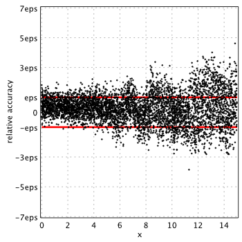
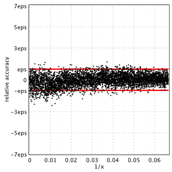
Actual accuracy of each approximation in terms of machine epsilon, eps = 2^-52 ˜ 2.22e-16, is plotted below:
(Please see our report on I₀(x) for technical details).

Blair & Edwards^[1]

{ 0 comments }

Rational Approximations for the Modified Bessel Function of the First Kind – `I₀(x)` for Computations with Double Precision

by Pavel Holoborodko on November 11, 2015

In this post we will study properties of rational approximations for modified Bessel function of the first kind $I_0(x)$ commonly used to compute the function values in double precision for real arguments. We compare the actual accuracy of each method, discuss ways for improvement and propose new approximation which delivers the lowest relative error.

BesselI Functions (1st Kind, n=0,1,2,3)

We consider following rational approximations: Blair & Edwards^[1], Numerical Recipes^[2], SPECFUN 2.5^[3], and Boost 1.59.0^[4]. All libraries use approximation of the same form, proposed in the work of Blair & Edwards^[1]:

(1) $\begin{alignat*}{2} I_0(x)&\approx P_n(x^2)/Q_m(x^2), \qquad &&|x| &\le 15.0 \\ x^{1/2} e^{-x} I_0(x)&\approx P_r(1/x)/Q_s(1/x), \qquad && x &\ge 15.0 \end{alignat*}$

where $P_*(x)$ and $Q_*(x)$ are polynomials of corresponding degrees.

{ 8 comments }

DevNotes #1. Multiplicative Operations with Complex Infinity

by Pavel Holoborodko on October 19, 2015

Every day we learn something new, gain experience and insights, collect interesting facts and tips. This process is especially intensive for software development when you deal with various algorithms, libraries, cross-platfrom development, performance optimization, etc.

To collect the summaries, ideas and facts I have been keeping development notes on a paper for a long time. But old style notebooks started to piled up and I have decided to write short posts for the blog instead. Hopefully it will be interesting for someone beside myself. Today will be the first attempt.
***

Different programming languages follow different rules in complex multiplicative operations when one of the operands is infinity. This came quite a surprise (thanks to Ciprian Necula who has drawn my attention to the issue).

All main mathematical packages (MATLAB, Mathematica and Maple) agreed on the following:

>> 1/(Inf+1i)                  % 1 
ans =
     0
 
>> Inf*(0+1i)
ans =
            0 +        Inf*i    % 2

{ 0 comments }

Solution of Poisson’s equation using Multiquadric Collocation Method in Extended Precision

by Pavel Holoborodko on August 9, 2015

Multiquadric (MQ) collocation method [1-3] is one of the most efficient algorithms for numerical solution of partial differential equations. It achieves exponential error convergence rate [4] and can handle irregular shaped domains well (in contrast to spectral methods).

Accuracy of the solution is controlled by shape parameter $\tiny{c}$ of MQ-radial basis function (RBF). With the increase of $c$ (flat function) accuracy also grows. However, in the same time, large $c$ leads to ill-conditioned system matrix. This effect received much attention from researchers [5-9] with focus on finding pre-conditioners, optimal values for $c$ , etc.

In this post we want to study the MQ collocation method by applying it to Poisson equation. To tackle the ill-conditioning and see the related effects we use different levels of precision.

At first, using arbitrary precision computations we evaluate empirical dependency of approximation error vs. shape parameter. In the second simulation we check how accuracy changes with grid refinement. See similar studies in [10-12].

Idea of running such tests was inspired by excellent book of Scott A. Sarra and Edward J. Kansa: Multiquadric Radial Basis Function Approximation Methods for the Numerical Solution of Partial Differential Equations (pdf). Original scripts from the book were modified to work with toolbox.

Problem

We consider two-dimensional Poisson problem on a unit disk domain (see section 3.1 in the book):

$u_{xx}+u_{yy}=f(x,y)$

The function $f(x,y)$ is specified so that the exact solution is

$u(x,y)=\frac{65}{65+\left(x-\frac{1}{5}\right)^2+\left(y+\frac{1}{10}\right)^2}$

Dirichlet boundary conditions are prescribed using the exact solution.

To solve the problem we apply asymmetric MQ RBF collocation method using the set of N near-equidistant centers generated in the domain:

{ 5 comments }

Citations Digest v.4

by Pavel Holoborodko on April 2, 2015

New toolbox citations found in Google Scholar or reported by the authors:

Books

Yair M. Altman, Accelerating MATLAB Performance: 1001 tips to speed up MATLAB programs, Chapman and Hall/CRC, 2015. Section 8.5.5 is devoted to the toolbox, its performance and (brief) comparison with similar libraries.
Shizgal, Bernie D., Spectral Methods in Chemistry and Physics: Applications to Kinetic Theory and Quantum Mechanics, Springer, 2015. Uses toolbox for verification of Laguerre quadrature weights & knots (toolbox has built-in function for generating the various Gauss-type quadrature).
C. A. Brebbia, A. H-D. Cheng, Boundary Elements and Other Mesh Reduction Methods, WITpress, Computational Mechanics, 2014. See chapter “Collocation and Optimization Initialization” by E. Kansa and L. Ling.
G. M. Carlomagno, D. Poljak, C. A. Brebbia Computational Methods and Experimental Measurements, Wit Transactions on Modelling and Simulation, 2015. See chapter “Strong form collocation: input for optimization” by E.J. Kansa.

{ 0 comments }

Version 3.8.0 release notes

by Pavel Holoborodko on February 12, 2015

Over last several months we have been focusing on making toolbox fast in processing the large matrices. Although many updates were released along the way (see full changelog) here we outline only the most important changes:

High-level dense linear algebra routines have been updated to use modern performance-oriented algorithms:
- Divide & Conquer for SVD [1, 2].
- Multi-shift QR for nonsymmetric eigenproblems [3, 4, 7].
- MRRR for Hermitian, symmetric and tridiagonal symmetric eigenproblems [5, 6].

All algorithms are implemented in quadruple as well as in arbitrary precision modes.

Most of the dense matrix algorithms have been enabled with parallel execution on multi-core CPUs. In future we plan to add support for GPU (at least for quadruple precision).
Many significant improvements have been made in toolbox architecture: low-level kernel modules are re-designed to minimize memory fragmentation, cache misses, copy-overhead in data exchange with MATLAB, etc.

All combined allows toolbox to reach the following results:

UPDATE (April 22, 2017): Timings for Mathematica 11.1 have been added to the table, thanks to test script contributed by Bor Plestenjak.

Matrix factorization in quadruple precision (500×500, 34 digits)
Factorization	Timing (sec)				Speed-up (times)
Factorization	MATLAB	Maple	Mathematica	Advanpix	Over MATLAB	Over Maple	Over Mathematica
A & B are pseudo-random real matrices (500×500):
[L,U] = lu(A)	249.13	85.16	15.12	0.47	534.38	182.67	32.42
[Q,R] = qr(A)	514.34	458.86	44.39	3.08	167.25	149.21	14.43
[U,S,V] = svd(A)	5595.26	4317.40	376.94	9.57	584.62	451.11	39.38
S = svd(A)	2765.11	645.60	56.96	2.98	927.17	216.48	19.10
[V,D] = eig(A)	21806.30	6060.90	584.86	33.75	646.05	179.57	17.33
lambda = eig(A)	3384.58	7822.30	205.46	23.55	143.70	332.11	8.72
[V,D] = eig(A,B)	n/a	11358.00	928.89	112.05	∞	101.36	8.29
lambda = eig(A,B)	n/a	5273.00	510.80	60.37	∞	87.34	8.46

Advanpix toolbox outperforms VPA by 500 times, Maple by 210 times and Wolfram Mathematica by 18 times in average.
Read more

{ 0 comments }

Advanpix vs.VPA – Array Manipulation Operations

by Pavel Holoborodko on November 14, 2014

New version of toolbox (≥3.7.2) has updated engine for array manipulation operations. We would like to show the improved timings and compare with previous version.

The very basic array manipulation operations (subscripted assignment, reference and concatenation) play crucial role in overall performance of the program. The poorly designed and implemented they might deteriorate the speed to the point when program actually spends more time in array indexing then computation itself.

MATLAB interpreter has extremely optimized basic operations for built-in “double” and “single” precision matrices. However situation is quite different when it comes to arrays of custom-defined types (like our multiple-precision class – mp).

As it was reported earlier [1], array manipulation functions provided by MATLAB for custom-defined types have absolutely unacceptable level of performance. We have investigated the issue and proposed our solution [1,2,3].

As a quick demo, here is comparison of sequential element-wise assignment (without pre-allocation):

% Variable-precision arithmetic (Symbolic Math Toolbox, MATLAB R2014a)
p = vpa('pi');
tic
for ii = 1:300
for jj = 1:300
   A(ii,jj) = p;
end
end
toc
 
Elapsed time is 848.209 seconds.
 
% Multiprecision Computing Toolbox >= 3.7.2
p = mp('pi');
tic
for ii = 1:300
for jj = 1:300
   A(ii,jj) = p;
end
end
toc
 
Elapsed time is 7.17263 seconds.

Symbolic Math Toolbox/VPA requires 14 minutes to just fill the 300x300 matrix!
Advanpix toolbox does the same in 7 seconds (118 times faster).

{ 0 comments }

Citations Digest v.3

by Pavel Holoborodko on February 3, 2014

Last few months were fruitful for toolbox citations:

R. Day, G. Vajente, and M. Pichot du Mezeray. Accelerated convergence method for the FFT simulation of coupled cavities.
J. M. Zhang, D. Braak and M. Kollar. Integrability and weak diffraction in a one-dimensional two-particle Hubbard model.
Francisco de la Hoz and Fernando Vadillo. The solution of two-dimensional advection–diffusion equations via operational matrices.
C. Siriteanu, S. Blostein, A. Takemura, H. Shin, S. Yousefi, S. Kuriki. Exact MIMO Zero-Forcing Detection Analysis for Transmit-Correlated Rician Fading.
(Ph.D. Thesis) Jonah A. Reeger. A Computational Study of the Fourth Painleve Equation and a Discussion of Adams Predictor-Corrector Methods.
Varun Shankar, Grady B. Wright, Robert M. Kirby, Aaron L. Fogelson. A Radial Basis Function (RBF)-Finite Difference (FD) Method for Diffusion and Reaction-Diffusion Equations on Surfaces.

Also toolbox was mentioned in following works:

Nicholas J. Higham and E. Deadman. A Catalogue of Software for Matrix Functions.
G. Beliakov. On fast matrix-vector multiplication with a Hankel matrix in multiprecision arithmetics.

Please let me know if you know other papers to be added to the list.

If you are using the toolbox in your research please cite it in your paper – this greatly supports future development.

{ 0 comments }

Advanpix vs. VPA vs. Maple – Dense Solvers and Factorizations

by Pavel Holoborodko on November 3, 2013

We continue to compare our toolbox with Maple and Symbolic Math Toolbox (VPA). This time we focus on main operations in dense linear algebra – solvers and factorizations.

Every case/routine is tested on a random 100 x 100 matrix. Average timing over ten tests is used.

Comparison of linear system solver (“\”) in quadruple precision
Matrix Type	Timing (sec)			Speed-up (times)
Matrix Type	VPA	Maple	Advanpix	Over VPA	Over Maple
General Real	0.99	0.58	0.02	42.22	24.67
Symmetric Positive Definite	0.99	0.63	0.01	77.10	49.31
General Complex	3.13	2.43	0.08	38.34	29.74
Hermitian Positive Definite	3.72	2.56	0.05	70.85	48.82

In average Advanpix solver is faster by 60 times over VPA and 40 times over Maple.

Comparison of matrix factorization in quadruple precision
Factorization	Timing (sec)			Speed-up (times)
Factorization	VPA	Maple	Advanpix	Over VPA	Over Maple
A is a general real matrix:
[L,U] = lu(A)	1.67	0.61	0.02	78.26	28.29
[Q,R] = qr(A)	3.46	2.60	0.08	44.44	33.46
[U,S,V] = svd(A)	30.85	20.99	0.30	101.66	69.17
S = svd(A)	15.88	2.51	0.07	223.54	35.35
[V,D] = eig(A)	57.25	29.54	0.72	79.20	40.86
lambda = eig(A)	21.21	26.90	0.34	62.31	79.01
A is a general complex matrix:
[L,U] = lu(A)	2.74	2.56	0.07	41.63	38.89
[Q,R] = qr(A)	10.99	11.39	0.25	43.38	44.99
[U,S,V] = svd(A)	65.56	57.53	0.81	80.96	71.04
S = svd(A)	25.28	10.22	0.26	98.24	39.71
[V,D] = eig(A)	89.30	129.54	2.85	31.34	45.46
lambda = eig(A)	33.14	113.99	1.29	25.67	88.32

As for factorizations, Advanpix toolbox outperforms VPA by 75 times and Maple by 50 times in average. Worth to note the massive speed gain of singular value decomposition (SVD) in particular.

{ 0 comments }

← Previous Entries

Next Entries →