Multiprecision Computing Toolbox User’s Manual
Contents
Installation
The Multiprecision Computing Toolbox is easily installed after following only a few brief steps.
Windows. After downloading the program allow it to run. Follow the step-by-step instructions of the installer to complete the installation process.
GNU Linux and Mac OSX. Installation instructions are provided upon trial version request for the platforms.
After installation we recommend completing the following steps:
- Add the destination folder where toolbox is installed to MATLAB’s search path. For Windows 7, this may look like the following:
>> addpath('C:\Users\[UserName]\Documents\Multiprecision Computing Toolbox\')
Alternatively, the
pathtoolcommand can also be used to permanently update MATLAB’s search path. - Run the test suite by using the following command:
>> mp.Test()
mp.Digits()     :   <- success
double()        :   <- success
colon()         :   <- success
plus()          :   <- success
minus()         :   <- success
times()         :   <- success
mtimes()        :   <- success
...
svd()           :   <- success
eig()           :   <- success
...
besselh()       :   <- success
hypergeom()     :   <- success
KummerM()       :   <- success
KummerU()       :   <- success
fft()           :   <- success
ifft()          :   <- success
Please report to us if there are any errors or other problems in the process.
Quick Start
Arbitrary precision numbers and matrices can be created with the new special function mp(), which stands for multiprecision:
>> mp.Digits(34);                   % Setup default precision to 34 decimal digits (quadruple).
>> format longG                     % Toolbox shows all digits in case of 'long' formats.

% Simple expressions evaluation in quadruple precision:
>> x = mp('pi/4')
x =
    0.7853981633974483096156608458198757

>> y = mp('sqrt(2)/2')
y =
    0.707106781186547524400844362104849

>> A = repmat(x,10,10);             % Create mp-matrix by scalar replication.
>> norm(y-cos(A))                   % Calculations are done with 34 digits precision.
ans =
    9.629649721936179265279889712924637e-35

% Assemble matrix row by row:
% (Butcher tableau for Gauss-Legendre method: https://goo.gl/izuFWg)
>> a1 = mp('[ 5/36              2/9-sqrt(15)/15   5/36-sqrt(15)/30 ]');
>> a2 = mp('[ 5/36+sqrt(15)/24  2/9               5/36-sqrt(15)/24 ]');
>> a3 = mp('[ 5/36+sqrt(15)/30  2/9+sqrt(15)/15   5/36             ]');
>> a = [a1;a2;a3];                  % Concatenate rows into final matrix

% Create mp-matrices by conversion from double
>> A = mp(rand(5));
>> B = mp(eye(5));
>> [V,D] = eig(A,B);
>> norm(A*V - B*V*D,1)/(norm(A,1) * norm(B,1))
ans =
    8.1433805952291741154581605524001229e-34

% Create sparse matrix with accumulation using triplets:
>> i = [6 6 6 5 10 10 9 9]';
>> j = [1 1 1 2 3 3 10 10]';
>> v = mp('[100 202 173 305 410 550 323 121]')';  % Prepare vector of nonzeros
>> S = sparse(i,j,v)                              % Form quadruple precision sparse matrix
S =
    (6,1)      475
    (5,2)      305
    (10,3)     960
    (9,10)     444
The argument to the constructor mp() can be a string with mathematical expression or usual MATLAB’s matrix of any numeric type (double, single, logical, int8, int16, int32, int64 or else). Complex numbers, n-dimensional arrays and sparse matrices are supported as well.
Constructor creates objects with default precision controlled by mp.Digits() routine. On toolbox startup default precision is assigned to 34 decimal digits which conforms to IEEE 174-2008 standard for quadruple precision.
mpstartup.m script in toolbox’s directory. It runs automatically at the beginning of every session before toolbox functionality is used. Default precision, number of guard digits and other settings can be adjusted there.Toolbox is capable of working with any level of precision – hardware configuration is the only limiting factor:
>> mp.Digits(300)
>> format longG

>> p = mp('pi')                      % Compute 300 digits accurate pi
p =
    3.14159265358979323846264338327950288419716939937510582097494459230
78164062862089986280348253421170679821480865132823066470938446095505822
31725359408128481117450284102701938521105559644622948954930381964428810
97566593344612847564823378678316527120190914564856692346034861045432664
821339360726024914128

>> mp.Digits(1000000)
>> tic; mp('pi'); toc;               % How about 10^6 digits of pi?
Elapsed time is 2.694803 seconds.    % Core 2 Quad 2.83GHz
Once are created, the new multiprecision numbers and matrices can be used in programs the same way as ordinary double precision objects:
% Solve generalized eigenproblem:
>> A = mp(diag([1:4]));
>> B = mp(diag([ones(1,3),0]));       % B is singular
>> [V,D] = eig(A,B)
V =
        1        0        0        0
        0        1        0        0
        0        0        1        0
        0        0        0        1
D =
        1          0          0          0
        0          2          0          0
        0          0          3          0
        0          0          0        Inf
% Solve unsymmetric system of linear equations:
>> A = rand(500,'mp');                     % Create random multiprecision matrix
>> b = rand(500,1,'mp');

>> tic; [L,U,P] = lu(A); toc;              % LU decomposition in quadruple precision
Elapsed time is 1.076820 seconds.

>> x = U\(L\(P*b));
>> norm(A*x-b,1)/(norm(A,1)*norm(b, 1))    % Check solution accuracy
ans =
    1.140092306011076796021008154729708e-34

>> y = A\b;                                % Solve the system by toolbox's mldivide operator
>> norm(A*y-b,1)/(norm(A,1)*norm(b, 1))
ans =
    1.140092306011076796021008154729708e-34
These examples show a basic principle of the MATLAB program porting to the computing with toolbox. In most cases, this is accomplished by substituting standard numeric objects with the analogous multiprecision entities. The rest of the code stays intact – computations are now completed using requested level of precision transparently to user.
double routines. Exactly the same code can be used, only input arguments should be changed to multiprecision type.Information on toolbox-specific routines can be obtained by the MATLAB help command: help mp.Digits, help mp.GaussLegendre, etc.)
MATLAB detects the multiprecision arguments and calls the appropriate function from toolbox automatically – no additional efforts are required from the user. This allows easy porting of existing scripts to do the computations with arbitrary precision almost without modifications.
The toolbox provides extended-precision equivalents to the majority of the commonly used MATLAB routines.
Every function in toolbox is implemented in multiple different modifications in order to support all special cases and features of MATLAB’s standard routines. For example, arbitrary precision eig(), svd(), ifft() and bicgstab() functions cover all of the following special cases:
Standard eigenproblem:
 e = eig(A)
 [V,D] = eig(A)
 [V,D,W] = eig(A)
All options are supported:
[___] = eig(A,balanceOption)
[___] = eig(A,B,algorithm)
[___] = eig(___,eigvalOption)
Generalized eigenproblem:
 e = eig(A,B)
 [V,D] = eig(A,B)
 [V,D,W] = eig(A,B)
Inverse fast Fourier transform:
 y = ifft(X)
 y = ifft(X,n)
 y = ifft(X,[],dim)
 y = ifft(X,n,dim)
 y = ifft(..., 'symmetric')
 y = ifft(..., 'nonsymmetric')
Singular value decomposition:
 s = svd(X)
 [U,S,V] = svd(X)
 [U,S,V] = svd(X,0)
 [U,S,V] = svd(X,'econ')
BiCGSTAB iterative solver for large/sparse matrices:
 x = bicgstab(A,b)
 bicgstab(A,b,tol)
 bicgstab(A,b,tol,maxit)
 bicgstab(A,b,tol,maxit,M)
 bicgstab(A,b,tol,maxit,M1,M2)
 bicgstab(A,b,tol,maxit,M1,M2,x0)
 [x,flag] = bicgstab(A,b,...)
 [x,flag,relres] = bicgstab(A,b,...)
 [x,flag,relres,iter] = bicgstab(A,b,...)
 [x,flag,relres,iter,resvec] = bicgstab(A,b,...)
Please refer to Function Reference page for a complete list of supported functions. All of them are capable of computing with arbitrary level of precision and support special cases and options of MATLAB.
Integer matrices can be converted directly to multiprecision using the
mp() constructor; floating-point numbers require more careful consideration:>> mp.Digits(50); >> format longG >> mp(1/3) % Accuracy is limited to double precision ans = % since 1/3 was evaluated in double precision first 0.33333333333333331482961625624739099293947219848633 >> mp('1/3') % Full precision accuracy ans = 0.33333333333333333333333333333333333333333333333333
Be aware that in some cases this may affect accuracy of the final result of computations:
>> mp.Digits(50);

>> sin(mp(pi))        % Double-precision pi reduces the accuracy of the result
ans =
     1.2246467991473531772260659322749979970830539012998e-16


>> sin(mp('pi'))      % Re-calculate pi with extended precision to have full accuracy
ans =
     7.3924557288138017054485818582464972262369629126385e-56
Generally, floating-point numbers should be re-calculated using high precision arithmetic from the onset, not converted from MATLAB as the accuracy is inherited. Please see More on Existing Code Porting for examples and more details.
In examples on the page we frequently use direct conversion of double matrices to mp-type. This is just for making demonstrations brief and simple, as it is not part of physical simulations or other meaningful computations. Please be careful in real-world applications.
More Examples
In this section we show several examples of toolbox usage in different fields. This reflects just the tiny portion of toolbox functionality, but we hope it will be helpful for understanding on how to apply toolbox in other situations.
Arbitrary Precision Gauss-Legendre Quadrature
Our first example illustrates one particular case of existing code porting to computing with extended precision.
The Gauss-Legendre quadrature’s nodes and weights can be calculated from the eigenvalues and eigenvectors of a Jacobi matrix, built from the coefficients of a 3-term recurrence relation of orthogonal Legendre polynomials. MATLAB code for the algorithm:
function [x,w] = gauss(N)
% GAUSS   Computes nodes and weights for Gauss-Legendre quadrature

    beta = .5./sqrt(1-(2*(1:N-1)).^(-2));
    T = diag(beta,1) + diag(beta,-1);
    [V,D] = eig(T);
    x = diag(D);
    [x,i] = sort(x);
    w = 2*V(1,i).^2;
end
Toolbox enables this program to calculate abscissae and weights with arbitrary precision, without any modifications to code:
>> N = 7;                               % Quadrature order
>> [x,w] = gauss(N);                    % Calculation with usual precision >> x

x =

        -0.949107912342758
        -0.741531185599394
        -0.405845151377397
    -1.15122081766977e-016
         0.405845151377397
         0.741531185599395
         0.949107912342758

>> mp.Digits(50);                       % Calculation with 50 digits accuracy >> [x,w] = gauss(mp(N));                % using the same MATLAB codex =
          -0.94910791234275852452618968404785126240077093767045
          -0.74153118559939443986386477328078840707414764714111
          -0.40584515137739716690660641207696146334738201409918
        1.0156505898350343455334038575175631139497748144399e-49
           0.40584515137739716690660641207696146334738201409949
           0.74153118559939443986386477328078840707414764714140
           0.94910791234275852452618968404785126240077093767061
How is this possible? During the program’s every function call, MATLAB detects the type of supplied arguments. Built-in functions are called for the numeric objects of standard double type. However, if an argument is a multiprecision number or matrix, MATLAB recognizes this and uses the functions provided by Multiprecision Computing Toolbox.
Thus, when we pass mp-number mp(N) to gauss(), MATLAB uses the high precision routines from the toolbox for all further mathematical operations: +, -, *, ./, colon(:), .^, diag(), eig() and sort().
It is important to note that MATLAB does a silent conversion of the floating-point constant 0.5 using the mp() constructor. Since 0.5 is a power of 2, it is exactly representable in binary format using the standard double type. As a result, direct conversion to extended precision is safe – no rounding error is introduced in a process. All other non-power-of-two constants should be re-computed in higher precision by the toolbox (e.g. 1/3 => mp('1/3') ).
mp.GaussLegendre, mp.GaussJacobi, mp.GaussLaguerre, mp.GaussHermite, mp.GaussChebyshevType[1|2] and mp.GaussGegenbauer.See Abscissas and Weights of Classical Gaussian Quadrature Rules for more details.
Linear Algebra (Dense matrices)
All linear algebra routines in toolbox are implemented in native C++/Assembler programming languages with heavy optimization for parallel execution on multi-core CPUs. We implement only state-of-the-art algorithms, as soon as they appear in LAPACK or published in papers.
Every routine (e.g. det, svd, eig, etc.) is a meta-algorithm which analyses the properties of the input matrix and applies the best suitable method for it.
Thus, for example, eigensolver uses multi-shift QR with aggressive deflation for unsymmetric matrices, MRRR or D&C for symmetric and tridiagonal matrices. The system solver \ handles much more additional cases, including positive definite, banded and triangular matrices.
Solve system of equations
% Solve ill-conditioned system of equations in double and extended precision:
>> A = hilb(30);
>> b = rand(30,1);

>> x = A\b;
'Warning: Matrix is close to singular or badly scaled. RCOND = 1.555731e-19.'

>> norm(A*x-b,1)/(norm(A,1)*norm(b,1))  % Computed solution is useless (as expected)
ans =
     1.094431774434172e+00

>> mp.Digits(50);
>> x = mp(A)\mp(b);    % Extended-precision solver is called automatically for mp-arguments

>> norm(A*x-b,1)/(norm(A,1)*norm(b,1))
ans =
    2.614621692258343564492414106947670112359638530373e-35
Although ill-conditioning has eaten up 15 digits of accuracy, extended precision is able to provide meaningful solution anyway.
Compute sensitive eigenvalues
% Compute eigenvalues of hexa-diagonal Toeplitz matrix of the form:
>> n = 7;
>> A = toeplitz([1,-1,zeros(1,n-2)],[1:5,zeros(1,n-5)])
A =
     1     2     3     4     5     0     0
    -1     1     2     3     4     5     0
     0    -1     1     2     3     4     5
     0     0    -1     1     2     3     4
     0     0     0    -1     1     2     3
     0     0     0     0    -1     1     2
     0     0     0     0     0    -1     1
The eigenvalues of the matrix (we call it “Circus matrix”) are invariant to transposition, so that eig(A)==eig(A.'). We verify this property below using the double and quadruple precision:
% MATLAB's double precision:
>> n = 100;
>> A = toeplitz([1,-1,zeros(1,n-2)],[1:5,zeros(1,n-5)]);
>> plot(eig(A),'k.'), hold on, axis equal
>> plot(eig(A.'),'ro')
% Quadruple precision (default in toolbox):
>> n = 100;
>> A = toeplitz([1,-1,zeros(1,n-2,'mp')],[1:5,zeros(1,n-5,'mp')]); % Numeric type changed to mp
>> plot(eig(A),'k.'), hold on, axis equal
>> plot(eig(A.'),'ro')
The eigenvalues of the original matrix are displayed in black, and the eigenvalues of the transposed – in red. They should coincide:


Similar examples can be found on the page Computing Eigenvalues in Extended Precision.
Besides the main routine eig, toolbox provides less common functions related to eigenproblems: condeig, schur, ordeig, ordqz, ordschur, poly, polyeig, qz, hess, balance, cdf2rdf and rsf2csf.
Compute subset of eigenvalues and eigenvectors
Toolbox implements EIGS routine for computing part of the eigenspectrum:
>> A = mp(delsq(numgrid('C',15)));
>> [V,D] = eigs(A,5,'SM');
>> diag(D)
ans =
        0.1334157995763293471169891415014640
        0.2675666637791856502089965060370031
        0.3468930344689260340608882099372852
        0.4787118036070204654965926915155679
        0.5519736907587845745371246531119098

>> norm(A*V-V*D,1)/norm(A,1)
ans =
    8.083857139088984628769006875834622e-33
It is based on Krylov-Schur iterative method with the support of usual features: standard and generalized eigenproblems, matrix and function handle inputs and various parts of the spectrum – 'SM', 'LM', 'SA', 'LA', 'SI', 'LI', 'SR' and 'LR'.
In case of handle inputs, routine MPEIGS should be called:
>> n = 1000;
>> A = mp(sprand(n,n,0.25));
>> F = precomputeLU(A);          % Toolbox's routine for computing and storing LU for efficient re-use.
>> Afun = @(x) F\x;
>> d = mpeigs(Afun,n,6,'SM')
d =
        -0.0288903225894439337485415046187058 +                                         0i
          0.189153427316800832137118934809178 -     0.04780063866543304346705036367999754i
          0.189153427316800832137118934809178 +     0.04780063866543304346705036367999754i
        -0.4537533919116012782272828193504341 +                                         0i
        -0.1404999441340245812855001335909667 -      0.5072737776980597238492023171446182i
        -0.1404999441340245812855001335909667 +      0.5072737776980597238492023171446182i
>> delete(F);
Matrix functions
Evaluation of matrix functions is closely related to Schur decomposition and eigenproblem in general. Naturally extended precision plays important role in the field as well. Toolbox provides all common routines – expm, sqrtm, logm, sinm, cosm, sinhm, coshm and funm for computing arbitrary matrix functions.
function r = test_expm(n)

  B = randn(n, n);
  [Q, ~] = eig(B);

  A = diag(logspace(-1, 1, n));
  A = Q * A * Q';
  [V, D] = eig(A);

  r = norm(expm(A) - V * diag(exp(diag(D))) / V,1) / norm(A,1); % relative error
end
Maximum relative error over 10 tests when run with double precision:
>> d=0; for i=1:10, d = max(d,test_expm(30)); end
>> d
d =
        3.1287663468819
Correct result can be obtained by using the quadruple precision:
>> d=0; for i=1:10, d = max(d,test_expm(mp(30))); end
>> d
d =
    9.131229307611786185465434992164817e-23
Linear Algebra (Sparse matrices)
Creation and manipulation
Similarly to dense case, multiprecision sparse matrices can be created in several ways.
% By conversion from double:
>> S = mp(sprand(100,100,0.001))
S =
    (17,8)     5.9486124934864759161712299828650430e-01
    (27,25)    4.3326919997192658851048463475308381e-01
    (28,27)    3.9133952726058496285332921615918167e-01
    (78,28)    3.2661940067820904864959175029071048e-01
    (62,48)    9.1338270917172348362100819940678775e-01

>> S = mp(speye(4,4))
S =
    (1,1)    1
    (2,2)    1
    (3,3)    1
    (4,4)    1
% By conversion from full matrix:
>> A = rand(100,'mp');
>> A(A < 0.999) = 0;
>> sparse(A)
ans =
    (93,3)     9.9938483953331447295909129024948925e-01
    (56,11)    9.9983373397479580191316017589997500e-01
    (36,15)    9.9944862738774264965257998483139090e-01
    (65,17)    9.9959431001853071840912434709025547e-01
    (53,30)    9.9911436902749595212469557736767456e-01
    (25,32)    9.9946412429982001146555603554588743e-01
    (91,33)    9.9980104396890978613043898803880438e-01
Or directly by using the special functions:
% Create from diagonals
>> n = 3;
>> e = ones(n,1,'mp');
>> S = spdiags([e -2*e e], -1:1, n, n)
S =
    (1,1)    -2
    (2,1)     1
    (1,2)     1
    (2,2)    -2
    (3,2)     1
    (2,3)     1
    (3,3)    -2
>> full(S)
ans =
        -2         1         0
         1        -2         1
         0         1        -2

% Build the same matrix by using 'sparse'
>> D = sparse(1:n,1:n,-2*ones(1,n,'mp'),n,n);
>> E = sparse(2:n,1:n-1,ones(1,n-1,'mp'),n,n);
>> S = E+D+E'
S =
    (1,1)    -2
    (2,1)     1
    (1,2)     1
    (2,2)    -2
    (3,2)     1
    (2,3)     1
    (3,3)    -2
>> full(S)
ans =
        -2         1         0
         1        -2         1
         0         1        -2
Toolbox provides the basic functionality for working with sparse matrices: element-wise access, indexing & assignment, concatenation and basic functions (nonzeros, spfun, spones, min/max, find, nnz, etc.). Arithmetic operations also support mixed type arguments (full-sparse) and compatible with MATLAB’s semantic (type of result, etc).
Direct solvers
System solver in toolbox (mldivide or \) relies on direct decompositions – LU, Cholesky and sparse QR, depending on problem to be solved. All of them are implemented in C++ and capable of working with arbitrary precision.
% Solve real symmetric positive definite problem, 5489x5489: http://goo.gl/IbQnST
>> S = mp(mmread('s3rmt3m1.mtx'));    % Load double matrix from file and convert to mp

>> nnz(S)*100/numel(S)                % percent of non-zero elements
ans =
         0.722453867804507

>> b = S*ones(size(S,2),1);           % Assume solution to be all ones

>> tic; x = S\b; toc;                 % Cholesky is used for SPD matrix
Elapsed time is 2.9553425 seconds.

>> norm(S*x-b,1)/norm(S,1)
ans =
    1.598989751907713334585798499335113e-31
The mmread routine is needed to read MatrixMarket matrices and it is provided here.
% Solve real unsymmetric problem, 5005x5005: http://goo.gl/W7kYDK
>> S = mp(mmread('sherman3.mtx'));   % Load double matrix from file and convert to mp

>> nnz(S)*100/numel(S)               % percent of non-zero elements
ans =
        0.0799719760758722

>> b = S*ones(size(S,2),1);

>> tic; x = S\b; toc;                % Sparse LU is used for asymmetric matrices
Elapsed time is 1.282938 seconds.

>> norm(S*x-b,1)/norm(S,1)
ans =
    8.284279608044027924347142865841002e-34
Timing examples for solving the test matrices from MatrixMarket and test scripts can be found on the pages: Direct Solvers for Sparse Matrices or Advanpix vs. Maple – Direct Sparse Solvers Comparison.
Iterative solvers
Toolbox includes following full-featured iterative solvers: BiCG, BiCGSTAB, BiCGSTABL, CGS, GMRES, MINRES and PCG.
All methods are capable of working with arbitrary precision sparse and dense matrices. Routines are implemented in different variants, support preconditionares, matrix and function handles as inputs. Please use them in your code, see Krylov Subspace Methods in Arbitrary Precision and Arbitrary Precision Iterative Solver – GMRES for more details.
But here we consider simple self-written conjugate gradient for illustrative purposes.
Let’s consider conjugate gradient iterative method and check how its convergence speed changes with precision. Here is very simple implementation (without preconditioning or else):
function [x, niter, flag] = conjgrad(A,b,s,tol,maxiter)
% CONJGRAD   Conjugate Gradients method (textbook implementation).
%
%    Input parameters:
%           A : Symmetric, positive definite NxN matrix
%           b : Right-hand side Nx1 column vector
%           s : Nx1 start vector (the initial guess)
%         tol : residual error tolerance for break
%               condition
%     maxiter : Maximum number of iterations to perform
%
%    Output parameters:
%           x : Nx1 solution vector
%       niter : Number of iterations performed
%        flag : 1 if convergence criteria fulfilled,
%               0 otherwise (= accuracy is not reached).

    x=s;
    r=b-A*x;
    p=r;
    rsold=r'*r;
    niter = 0;

    while true
        Ap=A*p;
        alpha=rsold/(p'*Ap);
        x=x+alpha*p;
        r=r-alpha*Ap;

        niter = niter + 1;
        if norm(r) < tol, flag = 1; break; end
        if niter == maxiter, flag = 0; break; end

        rsnew=r'*r;
        p=r+(rsnew/rsold)*p;
        rsold=rsnew;
    end
end
Ideally CG should produce exact solution in a number of steps no large than the size of the matrix. In a world of double precision floating-point arithmetic this obviously doesn’t work:
% Solve real symmetric positive definite matrix using CG, 237x237: http://goo.gl/FDqtRU
>> S = mmread('nos1.mtx');
>> b = S*ones(size(S,2),1);
>> x = rand(size(S,2),1)-0.5;

>> [y,iters,flag] = conjgrad(S,b,x,1e-10,5000);
>> iters
iters =
        3699
>> flag
flag =
     1
The method needs 15.6 times more iterations to reach the 1e-10 accuracy in double precision than theory dictates! Exactly the same routine can be used to solve the problem using quadruple precision:
>> mp.Digits(34);
>> [y,iters,flag] = conjgrad(mp(S),mp(b),mp(x),mp('1e-10'),5000); % Arguments are of mp-type now
>> iters
iters =
        1837
>> flag
flag =
     1
Two times less iterations needed, but still too many. Toolbox allows computing with any level of precision, e.g. let’s try 650 digits:
>> mp.Digits(650);
>> tic; [y,iters,flag] = conjgrad(mp(S),mp(b),mp(x),mp('1e-10'),5000); toc;
Elapsed time is 1.37769770653667 seconds.

>> iters
iters =
   237
>> flag
flag =
     1
Finally practice coincides with theory – method converged in 237 iterations = matrix size. Worth to note that high precision might actually give boost in performance, since much less number of iterations is required:
Iterations required to reach 1e-10 accuracy versus precision used in solver (CG, NOS1.mtx)

Numerical methods
Find function zeros
Find zeros of nonlinear function using fzero. Try double precision first:
>> f = @(x) sin(x).^2+cos(x).^2+2*cos(x).*cosh(x)+cosh(x).^2-sinh(x).^2;

>> fzero(f, 30)           % So far so good
ans =
          29.8449784514733

>> fzero(f, 50)           % fzero just returns the starting point for any x > 40 !?
ans =
    50

>> fzero(f, 80)
ans =
    80
Here is plot of the function produced by MATLAB in double precision:

Do the same but with 50-digits of precision:
>> mp.Digits(50);

>> fzero(f,mp('50'))
ans =
    48.694686130641795196169549468320090302693738489349

>> fzero(f,mp('80'))
ans =
    80.110612666539727516937363111757401732175389957391

>> x = mp(0):mp('.1'):mp('60');
>> y = f(x);
>> plot(x,y)
>> axis([0 60 -1e+10 1e+10]);

MATLAB is not able to overcome the cancellation errors in computing function zeros, whereas elevated precision does provide the correct results.
Polynomial roots
Finding roots of the Wilkinson’s polynomial using double precision:
>> z=1:25; p=poly(z); r=roots(p)
r =
  24.8949 + 0.3929i
  24.8949 - 0.3929i
  23.3980 + 1.6599i
  23.3980 - 1.6599i
  21.2414 + 2.6833i
  21.2414 - 2.6833i
  18.7294 + 3.1668i
  18.7294 - 3.1668i
  16.1915 + 3.0915i
  16.1915 - 3.0915i
  13.8433 + 2.5822i
  13.8433 - 2.5822i
  11.7833 + 1.8021i
  11.7833 - 1.8021i
  10.0214 + 0.8985i
  10.0214 - 0.8985i
   8.7436 + 0.0000i
   8.0539 + 0.0000i
   6.9956 + 0.0000i
   6.0003 + 0.0000i
   5.0000 + 0.0000i
   4.0000 + 0.0000i
   3.0000 + 0.0000i
   2.0000 + 0.0000i
   1.0000 + 0.0000i

>> norm(z-flip(r'),Inf)
ans =
    3.2497
…and using quadruple precision:
>> mp.Digits(34);
>> z=mp(1:25); p=poly(z); r=roots(p)
r =

         24.99999999999999999998747884729626
         23.99999999999999999972707494735599
         23.00000000000000000413806455260104
         21.99999999999999997542594633350117
         21.00000000000000008761543344145269
         19.99999999999999978485063601064847
         19.00000000000000038917245147571848
          17.9999999999999994611237110991513
          17.0000000000000005847139434974281
         15.99999999999999949573405863767598
         15.00000000000000034835761470681007
         13.99999999999999980666078729854471
         13.00000000000000008611457075304565
         11.99999999999999996936046988869544
         11.00000000000000000863956001512734
         9.999999999999999998090523293768979
         9.000000000000000000326216861348089
         7.999999999999999999957632911734256
         7.000000000000000000004099106384922
         5.999999999999999999999712940349484
         5.000000000000000000000013775121721
         3.999999999999999999999999601328278
         3.000000000000000000000000004907469
         2.000000000000000000000000000004614
        0.9999999999999999999999999999998554

>> norm(z-flip(r'),Inf)
ans =
    5.847139434974281026037891270188779e-16
Numerical integration
Numerical integration using the adaptive Gauss-Kronrod quadrature:
>> f = @(x)(10*sin(x+exp(x))./(x-3*atan(x-5)));
>> [q,errbnd] = quadgk(f,mp(0),mp(10),'RelTol',mp('1e-10'),'MaxIntervalCount',10000)
q =
    0.859792389192094816413248930451348
errbnd =
    5.741317225977969319337426215581556e-11
The quadgk routine provided in toolbox computes Gauss-Kronrod coefficients for the requested precision and then runs adaptive integration algorithm.
If you are interested in more details on how to compute the coefficients in arbitrary precision please take a look on the page: Gauss-Kronrod Quadrature Nodes and Weights.
Ordinary differential equations
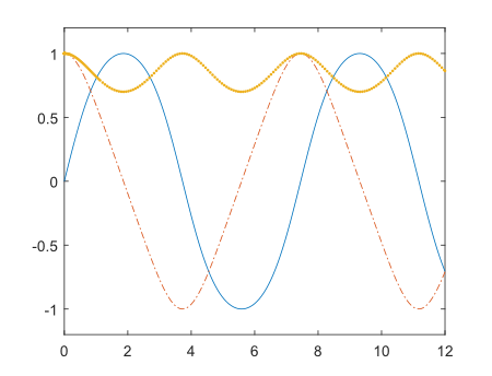
Solve nonstiff differential equations using ode113 (toolbox also provides ode45 and ode15s):
function dy = rigid(t,y)
 dy = mp(zeros(3,1));
 dy(1) = y(2) * y(3);
 dy(2) = -y(1) * y(3);
 dy(3) = mp('-0.51') * y(1) * y(2);
end

>> mp.Digits(34);
>> options = odeset('RelTol',mp('1e-10'),'AbsTol',repmat(mp('1e-10'),1,3));
>> [T,Y] = ode113(@rigid,mp('[0 12]'),mp('[0 1 1]'),options);

>> plot(T,Y(:,1),'-',T,Y(:,2),'-.',T,Y(:,3),'.')
Solve system of nonlinear equations (fsolve)
Toolbox provides full-featured fsolve, including sparse formulation, Jacobian and three algorithms of optimization: Levenberg-Marquardt, trust-region-dogleg and trust-region-reflective. All options and special cases are covered:
 x = fsolve(fun,x0)
 x = fsolve(fun,x0,options)
 x = fsolve(problem)
 [x,fval] = fsolve(fun,x0)
 [x,fval,exitflag] = fsolve(...)
 [x,fval,exitflag,output] = fsolve(...)
 [x,fval,exitflag,output,jacobian] = fsolve(...)
Quick start example for demonstration:
function test_fsolve
x0 = mp([-5; -5]);
options = optimset('Display','iter', 'TolFun', mp('eps'),...
                                       'TolX', mp('eps'),...
                                  'Algorithm','levenberg-marquardt');

[x,fval,exitflag,output] = fsolve(@myfun,x0,options)

    function F = myfun(x)
        F = [2*x(1) - x(2) - exp(-x(1));
              -x(1) + 2*x(2) - exp(-x(2))];
    end
end
Output:
>> mp.Digits(34);
>> test_fsolve

                                        First-Order                    Norm of
 Iteration  Func-count    Residual       optimality      Lambda           step
     0           3         47071.2        2.29e+04         0.01
     1           6         6527.47        3.09e+03        0.001        1.45207
     2           9         918.374             418       0.0001        1.49186
     3          12         127.741            57.3        1e-05        1.55326
     4          15         14.9153            8.26        1e-06        1.57591
     5          18        0.779056            1.14        1e-07        1.27662
     6          21      0.00372457          0.0683        1e-08       0.484659
     7          24      9.2164e-08        0.000336        1e-09      0.0385554
     8          27     5.66104e-17        8.34e-09        1e-10    0.000193709
     9          30     2.35895e-34         1.7e-17        1e-11    4.80109e-09
    10          33     1.70984e-51        4.58e-26        1e-12    9.80056e-18
    11          36      1.8546e-68        1.51e-34        1e-13    2.63857e-26

Equation solved.

fsolve completed because the vector of function values is near zero
as measured by the selected value of the function tolerance, and
the problem appears regular as measured by the gradient.

x =
        0.56714
        0.56714
fval =
        9.6296e-35
        9.6296e-35
exitflag =
     1
output =
       iterations: 11
        funcCount: 36
         stepsize: [1x1 mp]
     cgiterations: []
    firstorderopt: [1x1 mp]
        algorithm: 'levenberg-marquardt'
          message: 'Equation solved.

Equation solved. The sum of squared function values, r = 1.854603e-68, is less
than sqrt(options.TolFun) = 1.387779e-17. The relative norm of the gradient of
r, 6.583665e-39, is less than 1e-4*options.TolFun = 1.925930e-38.

Optimization Metric                                        Options
relative norm(grad r) =   6.58e-39           1e-4*TolFun =   2e-38 (selected)
r =   1.85e-68                             sqrt(TolFun) =  1.4e-17 (selected)
Symbolic Math Toolbox (VPA) vs. Multiprecision Computing Toolbox
There is a huge difference in performance of linear algebra algorithms:
>> A = rand(500)-0.5;

% VPA (MATLAB R2014a x64):
>> digits(25);                       % Equivalent to 34-digits, as 9 guard digits are used.
>> tic; [U,S,V] = svd(vpa(A)); toc;
Elapsed time is 5595.266780 seconds. % 1.5 hours

>> norm(A-U*S*V',1) / norm(A,1)
ans =
    6.674985970577584310073452e-33

% Advanpix Multiprecision Toolbox:
>> mp.Digits(34);
>> tic; [U,S,V] = svd(mp(A)); toc;   % We use parallel divide & conquer algorithm for SVD
Elapsed time is 13.831470 seconds.   % 400 times faster

>> norm(A-U*S*V',1) / norm(A,1)
ans =
    3.651822672021783818071962654139701e-33
Even in basic operations like elementary functions:
% VPA (MATLAB R2016b x64):
>> digits(25);
>> A = vpa(200*(rand(2000)-0.5));

>> tic; log(A); toc;
Elapsed time is 1161.7028 seconds.

>> tic; tan(A); toc;
Elapsed time is 1261.6516 seconds.

>> tic; besselj(0,A); toc;
Elapsed time is 7273.5572 seconds.

% Advanpix Multiprecision Toolbox:
>> mp.Digits(34);
>> A = mp(200*(rand(2000)-0.5));

>> tic; log(A); toc;
Elapsed time is 0.2334 seconds.   % ~5000 times faster

>> tic; tan(A); toc;
Elapsed time is 0.1704 seconds.   % ~7000 times faster

>> tic; besselj(0,A); toc;
Elapsed time is 0.7592 seconds.   % ~10000 times faster
Or in trivial array manipulation (e.g. vertical concatenation):
% VPA (MATLAB R2016a x64):
>> digits(25);
>> B = vpa(rand(200,200));
>> tic; for k=1:2000, [B; B]; end; toc;
Elapsed time is 267.514101 seconds.

% Advanpix Multiprecision Toolbox:
>> mp.Digits(34);
>> A = mp(rand(200,200));
>> tic; for k=1:2000, [A; A]; end; toc;
Elapsed time is 3.724525 seconds.        % 72 times faster
eig(A,B), fsolve, schur, fft/ifft, qz, quadgk, ordschur, ode45, ordqz, etc. to entire fields – n-dim arrays and sparse matrices.VPA loses accuracy while computing basic special functions, e.g.:
% VPA (MATLAB R2016b x64)
>> digits(34);
>> bessely(0,vpa(1000*i))
ans =
-2.54099907...376797872e381 + 2.485686096075864174562771484145676e432i   % Huge real part?

% Advanpix Multiprecision Toolbox:
>> bessely(0,mp(1000*i))
ans =
-1.28057169...387105221e-436 + 2.485686096075864174562771484145677e+432i % Not really
Overall MATLAB has serious issues with accurate computation of special functions even in double precision.
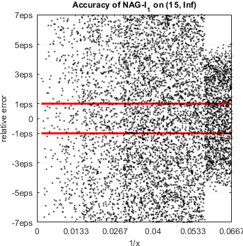
In case of Bessel functions of the first and second kind Yn(x) and Jn(x) – MATLAB suffers from catastrophic accuracy loss near zeros of the functions. Red lines show the expected limits of relative error for double precision:
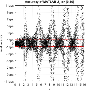
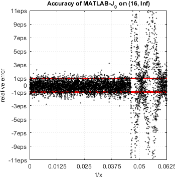
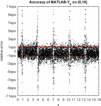
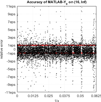
MATLAB’s functions bessely(n,x) and besselj(n,x) give no single correct digit in neighborhood of zeros of Yn(x) and Jn(x).
In case of modified Bessel functions MATLAB provides non-uniform accuracy (depending on argument range) and actually gives the highest error among mathematical libraries. For example, relative accuracy in terms of machine epsilon for  might reach the
 11.5eps near  :
:
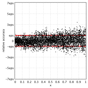
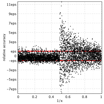
Please refer to the reports: K0(x), K1(x), I0(x) and I1(x) for more details on modified functions.
Built-in Hankel functions in MATLAB suffers from accuracy loss as well:
>> format longE;
>> mp.FollowMatlabNumericFormat(true);

>> besselh(-3.5,2,0.164675)
ans =
     -6.6224e+03 - 6.6224e+03i  % imaginary part is completely wrong

>> besselh(mp('-3.5'),2,mp('0.164675'))   % true value
ans =
    -6.6223671360899468166443367304659844e+03 - 1.37497005491890762469900821660588647e-05i
Same for gamma (and many other functions) in MATLAB:
% Example is from:
% S.M. Rump. Verified sharp bounds for the real gamma function over the entire floating-point range.
% Nonlinear Theory and Its Applications (NOLTA), IEICE, Vol.E5-N,No.3, July, 2014.

>> format longE;
>> mp.FollowMatlabNumericFormat(true);

>> x = -1+eps
x =
    -9.999999999999998e-01

>> gamma(mp(x))   % true value, quadruple precision
ans =
    -4.5035996273704964227843350984674649e+15

>> gamma(x)       % built-in function gives no correct digits at all
ans =
    -3.108508488097334e+15
To be fair, accuracy loss is endemic issue of numerical libraries, commercial or open source. For example, relative accuracy plots for I1(x) of NAG libraries:
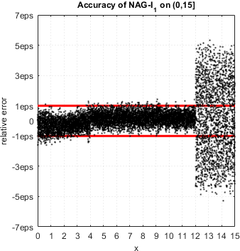
NAG demonstrates serious accuracy degradation for  :
:
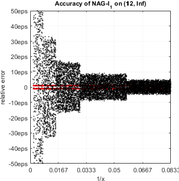
Actually relative error can be as high as 257eps.
Last but not the least issue with Symbolic Math Toolbox is that it doesn’t follow semantic of MATLAB’s standard functions. For example, it has no support for n-dimensional arrays in basic functions like max, min, sum, mean, etc.:
>> A = rand(2,2,2);

% Double precision
>> max(A)
ans(:,:,1) =
         0.602843089382083         0.711215780433683
ans(:,:,2) =
         0.296675873218327         0.424166759713807

>> sum(A)
ans(:,:,1) =
         0.865054837162928         0.932962514450923
ans(:,:,2) =
         0.414093524074133          0.74294506163969

% Advanpix Multiprecision Toolbox:
>> max(mp(A))
ans(:,:,1) =
        0.6028430893820829750140433134220075        0.7112157804336829425295718465349637
ans(:,:,2) =
        0.2966758732183268909565754256618675        0.4241667597138072398621488900971599

>> sum(mp(A))
ans(:,:,1) =
         0.865054837162928413896167967322981        0.9329625144509230416645095829153433
ans(:,:,2) =
        0.4140935240741328016156330704689026        0.7429450616396895412663070601411164

% VPA (MATLAB R2016a x64):
>> max(vpa(A))
'Error using sym/max (line 92)'
'MAX for higher-dimensional symbolic arrays is not supported.'
'Only scalars, vectors and matrices are valid input.'

>> sum(vpa(A))
'Error using symengine (line 59)'
'Input arguments must be two-dimensional.'
'Error in sym/privUnaryOp (line 909)'
'            Csym = mupadmex(op,args{1}.s,varargin{:});'
'Error in sym/sum (line 56)'
'    s = privUnaryOp(A, symobj::prodsum, _plus);'
More on Existing Code Porting
Smooth transition (ideally without modifications) of existing code to arbitrary precision is the main goal of the Multiprecision Computing Toolbox. However, there is an important case to be aware of.
Floating-point numerical constants in the code, such as 1/3, pi, sin(pi/3), sqrt(2)/2, eps, realmin, realmax, should be calculated using multiprecision arithmetic – mp('1/3'), mp('pi'), mp('sin(pi/3)'), mp('sqrt(2)/2'), mp('eps'), eps('mp'), realmin('mp'), realmax('mp'). Otherwise, MATLAB will evaluate these numbers with its standard precision first, and this might affect the overall accuracy of computations as well as final result.
>> mp.Digits(50);

>> mp(1/3)            % Accuracy is limited to double precision
ans =                 % since 1/3 was evaluated in double precision first
    0.33333333333333331482961625624739099293947219848633

>> mp('1/3')          % Full precision accuracy
ans =
    0.33333333333333333333333333333333333333333333333333

>> mp(1e+500)         % 1e+500 goes beyond double precision limits
ans =
    Inf

>> mp('1e+500')
ans =
    1e+500
Be aware that in some cases this may affect accuracy of the final result of computations:
>> mp.Digits(50);

>> sin(mp(pi))        % Double-precision pi reduces the accuracy of the result
ans =
     1.2246467991473531772260659322749979970830539012998e-16


>> sin(mp('pi'))      % Re-calculate pi with extended precision to have full accuracy
ans =
     7.3924557288138017054485818582464972262369629126385e-56
Extra-care should be taken to the stopping criteria of various iterative algorithms. Most likely it should be changed to allow more iterations and use machine epsilon matching to precision used.
Following function is from Chebfun, it is one of the many used in computing nodes & weights of Gauss-Laguerre quadrature:
function [x1, d1] = alg3_Lag(n, xs)
[u, up] = eval_Lag(xs, n);
theta = atan(sqrt(xs/(n + .5 - .25*xs))*up/u);
x1 = rk2_Lag(theta, -pi/2, xs, n);

% Newton iteration
step = inf;
l = 0;
while ( (abs(step) > eps || abs(u) > eps) && (l < 200) )
    l = l + 1;
    [u, up] = eval_Lag(x1, n);
    step = u/up;
    x1 = x1 - step;
end

%[ignored, d1] = eval_Lag(x1, n);
[~, d1] = eval_Lag(x1, n);
end
Assuming that input parameter xs is passed as mp-number, the routine will run in multiprecision mode. But still we need to do few changes to the code (changed lines are highlighted):
function [x1, d1] = alg3_Lag(n, xs)
[u, up] = eval_Lag(xs, n);
theta = atan(sqrt(xs/(n + .5 - .25*xs))*up/u);
x1 = rk2_Lag(theta, -mp('pi/2'), xs, n);       % (1) Use accurate pi
% Newton iteration
step = inf;
l = 0;

% (2) Use correct machine epsilon and increase allowable number of iterations:
while ( (abs(step) > mp('eps') || abs(u) > mp('eps')) && (l < 2000) )    l = l + 1;
    [u, up] = eval_Lag(x1, n);
    step = u/up;
    x1 = x1 - step;
end

%[ignored, d1] = eval_Lag(x1, n);
[~, d1] = eval_Lag(x1, n);
end
Now stopping criteria is capable of working with arbitrary precision (maximum number of iterations is an open question, probably it needs to be found empirically for every level of precision or omitted altogether).
Please check the article How to write precision independent code in MATLAB for more ideas on the process.
