Rational Approximations for the Modified Bessel Function of the Second Kind – `K₁(x)` for Computations with Double Precision

by Pavel Holoborodko on January 5, 2016

In this post we will consider minimax rational approximations used for computation of modified Bessel functions of the second kind – $K_1(x)$ . We will follow our usual workflow – we study properties of the existing methods and then propose our original approximations optimized for computations with double precision.

We try to keep the post brief and stick to results. Detailed description of our methodology can be found in previous reports of the series: K₀(x), I₀(x) and I₁(x).

In their pioneering work^[1], Blair & Russon proposed the following approximation forms for $K_0(x)$ :

For small arguments, $x<1$ :

(1) $\begin{alignat*}{2} K_1(x)-\ln(x)I_1(x)-1/x&\approx xP_n(x^2)/Q_m(x^2)\\ I_1(x)&\approx xP_r(x^2)/Q_s(x^2), \end{alignat*}$
For large values of $x\geqslant1$ :

(2) $\begin{equation*} x^{1/2}e^x K_1(x) \approx P_v(1/x)/Q_u(1/x) \end{equation*}$

All software libraries relying on rational approximations for computing $K_1(x)$ use (1) and (2) with small variations in coefficients of polynomials $P_*(x)$ and $Q_*(x)$ .

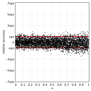
Relative accuracy shown below is measured in terms of machine epsilon ( eps = 2^-52 ˜ 2.22e-16) against “true” values of the function computed in quadruple precision by Maple. Red lines show natural limits for relative error we expect for double precision computations.

Blair & Russon^[1], Boost 1.59.0^[2] and SPECFUN 2.5^[3]

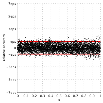
Boost and SPECFUN use the same coefficients from original report of Blair & Russon.

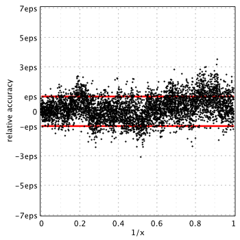
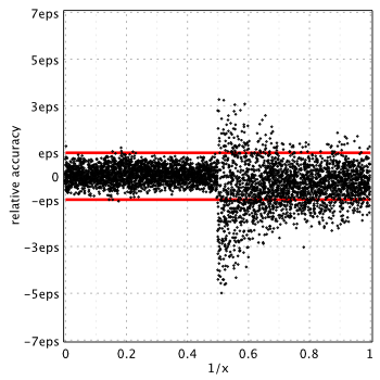
Numerical Recipes, 3rd edition, 2007^[4]

Strangely enough Numerical Recipes delivers good accuracy for $K_1(x)$ , $x<1$ , whereas it shows very poor performance for all other functions – $K_0(x)$ , $I_0(x)$ and $I_1(x)$ .

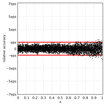
GNU GSL 2.0^[5]
(GSL uses Chebyshev series)

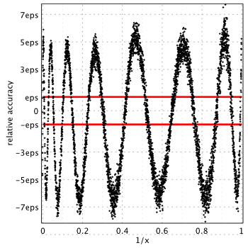
MATLAB 2015a^[6]
(MATLAB uses Chebyshev series)

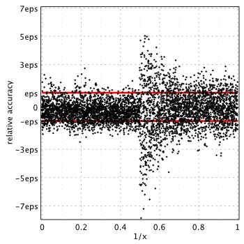
Similar to K₀(x), MATLAB provides the lowest accuracy for $x\in[0,2]$ compared to all other libraries. Relative error is up to 10.14eps near the $x=2$ . GSL and MATLAB use Chebyshev expansion for computations and apparently both suffer from similar issues (incorrectly rounded Chebyshev coefficients as GSL source code revealed).

Peak relative error^† in terms of machine epsilon – $K_1$
Method/Software	$x\in[0,1)$	$x \in[1,\infty)$
Minimax Rational Approximations:
Blair & Russon/Boost/SPECFUN	2.06	3.77
Numerical Recipes, 2007	1.95	8.51
Refined – (4), (5)	1.63	2.25
Chebyshev Expansions:
GNU GSL 2.0	2.95	7.11
MATLAB 2015a	2.83	10.14

†computed over 50K uniformly distributed random samples in each interval

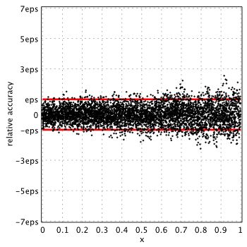
Refined Approximations

In a search for better accuracy we use extended approximation form for $I_1(x)$ near zero:

(3) $\begin{alignat*}{2} K_1(x)-\ln(x)I_1(x)-1/x&\approx xP_n(x^2)/Q_m(x^2)\\ I_1(x)&\approx \frac{x}{2}\left(1+\frac12\left[\frac{x}{2}\right]^2+\left[\frac{x}{2}\right]^4\frac{P_r([x/2]^2)}{Q_s([x/2]^2)}\right), \end{alignat*}$

This form reflects behavior of $I_1(x)$ for small arguments well and showed good results in our previous study. For large arguments we use the same formula as in (2).

Instead of using pure approximation error (usually computed in extended precision when rounding errors are ignored), we use additional criteria to find the optimal approximations. Highest priority is assigned to the actual accuracy delivered by schema in double precision. In other words, we take into account conditioning of the approximation in double precision.

This allows us to find approximations which are much more suitable for double precision computations with following properties:

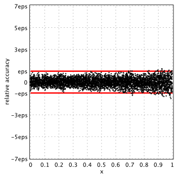
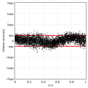
Maximum error is 1.63eps for small arguments and 2.25eps for $x\ge1$ .

Final expressions for optimal approximations:

For small arguments, $x<1$ :

(4) $\begin{alignat*}{2} K_1(x)-\ln(x)I_1(x)-1/x&\approx xP_8(x^2)\\ I_1(x)&\approx \frac{x}{2}\left(1+\frac12\left[\frac{x}{2}\right]^2+\left[\frac{x}{2}\right]^4 P_{5}([x/2]^2)\right) \end{alignat*}$
For large arguments, $x\ge1$ :

(5) $\begin{equation*} x^{1/2}e^x K_1(x) \approx P_{22}(x^{-1})/Q_2(x^{-1}) \end{equation*}$

Coefficients of the polynomials:

n	$P_{8}(x)$
0	-3.0796575782920622440538935e-01
1	-8.5370719728650778045782736e-02
2	-4.6421827664715603298154971e-03
3	-1.1253607036630425931072996e-04
4	-1.5592887702110907110292728e-06
5	-1.4030163679125934402498239e-08
6	-8.8718998640336832196558868e-11
7	-4.1614323580221539328960335e-13
8	-1.5261293392975541707230366e-15

n	$P_{5}(x)$
0	8.3333333333333325191635191e-02
1	6.9444444444467956461838830e-03
2	3.4722222211230452695165215e-04
3	1.1574075952009842696580084e-05
4	2.7555870002088181016676934e-07
5	4.9724386164128529514040614e-09

n	$P_{22}(x)$
0	1.0234817795732426171122752e-01
1	9.4576473594736724815742878e-01
2	2.1876721356881381470401990e+00
3	6.0143447861316538915034873e-01
4	-1.3961391456741388991743381e-01
5	8.8229427272346799004782764e-02
6	-8.5494054051512748665954180e-02
7	1.0617946033429943924055318e-01
8	-1.5284482951051872048173726e-01
9	2.3707700686462639842005570e-01
10	-3.7345723872158017497895685e-01
11	5.6874783855986054797640277e-01
12	-8.0418742944483208700659463e-01
13	1.0215105768084562101457969e+00
14	-1.1342221242815914077805587e+00
15	1.0746932686976675016706662e+00
16	-8.4904532475797772009120500e-01
17	5.4542251056566299656460363e-01
18	-2.7630896752209862007904214e-01
19	1.0585982409547307546052147e-01
20	-2.8751691985417886721803220e-02
21	4.9233441525877381700355793e-03
22	-3.9900679319457222207987456e-04

n	$Q_{2}(x)$
0	8.1662031018453173425764707e-02
1	7.2398781933228355889996920e-01
2	1.4835841581744134589980018e+00

text

Conclusion

We have derived new rational approximations for the modified Bessel function of the second kind – $K_1(x)$ . On the contrary to existing methods we minimize the actual error delivered by approximation in double precision. Proposed methods provide highest relative accuracy among all publicly available approximations (published and/or implemented in software).

MATLAB suffers from accuracy loss near zero and should be avoided if accuracy is of high priority.

References

Russon A.E., Blair J.M., Rational function minimax approximations for the modified Bessel functions $K_0(x)$ and $K_1(x)$ , AECL-3461, Chalk River Nuclear Laboratories, Chalk River, Ontario, October 1969.
Boost – free peer-reviewed portable C++ source libraries. Version 1.59.0. Boost: Modified Bessel function of the second kind.
Cody W.J., Algorithm 715: SPECFUN – A Portable FORTRAN Package of Special Function Routines and Test Drivers, ACM Transactions on Mathematical Software, Volume 19, Number 1, March 1993, pages 22-32. SPECFUN: Modified Bessel function of the second kind.
Press, William H. and Teukolsky, Saul A. and Vetterling, William T. and Flannery, Brian P. Numerical Recipes 3rd Edition: The Art of Scientific Computing, 2007, Cambridge University Press, New York, USA.
M. Galassi et al, GNU Scientific Library Reference Manual, 3rd Edition (January 2009), ISBN 0954612078.
MATLAB 2015a, The MathWorks, Inc., Natick, Massachusetts, United States.

{ 2 comments… read them below or add one }

John Maddock January 24, 2017 at 7:30 pm

I thought you would like to know that I’ve just implemented something similar to this for Boost.Math.

However it’s actually possible to do a little better, consider (5) for a moment, it turns out that K1(x)x^1/2 e^x is approximately constant for x > 1, and therefore there’s an old trick we can use – to replace P22/Q2 by C+R(x) where C is an arbitrary constant chosen to be the approximate value of the function over the range in question (truncated to an exact binary value), and R(x) is a rational approximation optimised for low *absolute* error compared to C. Now as long as the error with which we evaluate R(x) is small compared to C, we effectively “erase” the error when we perform the addition. Of course we may still round incorrectly as a result of the erroneous bits from R(x), so the error is slightly more than 0.5ulp, but we should be close. Add in 0.5ulp from the other 2 terms and we should achieve an overall maximum error just slightly more than 1.5ulp ~ 1.5eps.

I’m not sure how far you minimised P22/Q2 but another observation is that interpolated solutions for (5) are really quite far from minimax solutions. For example P22/Q2 interpolated is just accurate enough for double precision (error 8e-17), while the minimax solution is nearer to 3e-18. Which is my way of saying that many fewer terms can be used 😉

Using a P8/Q8 solution:

P = {    -1.97028041029226295e-01,
    -2.32408961548087617e+00,
    -7.98269784507699938e+00,
    -2.39968410774221632e+00,
    3.28314043780858713e+01,
    5.67713761158496058e+01,
    3.30907788466509823e+01,
    6.62582288933739787e+00,
    3.08851840645286691e-01,
  }

Q = {    1.00000000000000000e+00,
    1.41811409298826118e+01,
    7.35979466317556420e+01,
    1.77821793937080859e+02,
    2.11014501598705982e+02,
    1.19425262951064454e+02,
    2.88448064302447607e+01,
    2.27912927104139732e+00,
    2.50358186953478678e-02,
  }

and C = 1.45034217834472656

Yielded an approximation with a peek experimental error for K1 of 1.6eps. Just as importantly, it’s much faster to execute: the issue with large polynomials is that each arithmetic operation is dependent on the previous result which completely stalls the processor pipeline. You can mitigate this somewhat by using a second order Horner scheme, but even that doesn’t seem to be enough to keep the pipeline full, here’s the approximate performance results I obtained on Intel-x64 (all relative times):

P22/Q2 (Horner) 1.12
P22/Q2 (2nd order Horner) 0.743
P8/Q8 (Horner) 0.41
P8/Q8 (2nd order Horner) 0.38

[aside – we can of course go even further with rational approximations and use SIMD instructions to evaluate the 2 polynomials in parallel.]

Similar arguments apply to(4) where your P5 and P8 are being added to terms > 1, so these need only be optimised for low absolute error, similarly for K0. Both functions also extend to 128-bit precision fairly easily using these techniques BTW.

Apologies for the long post, but hopefully someone will find this useful, for the record, Boost’s code is here:

https://github.com/boostorg/math/blob/develop/include/boost/math/special_functions/detail/bessel_k0.hpp
and here:
https://github.com/boostorg/math/blob/develop/include/boost/math/special_functions/detail/bessel_k1.hpp

Pavel Holoborodko January 25, 2017 at 12:15 pm

Thank you for the wealth of information and congratulations on results!
I am sure it will be useful for many people as well.

Just for information, here is improvement of max relative error on 1M of random points in each interval:

--> BOOST 1.59.0 /MODIFIED BESSEL
BOOST/I0(x): [0,16] ->       6.13eps	[16,Inf] ->       3.04eps
BOOST/I1(x): [0,16] ->       5.44eps	[16,Inf] ->       3.03eps
BOOST/I2(x): [0,16] ->      12.16eps	[16,Inf] ->       9.47eps
BOOST/I3(x): [0,16] ->      12.06eps	[16,Inf] ->       9.75eps
BOOST/I4(x): [0,16] ->      12.39eps	[16,Inf] ->      10.35eps
BOOST/K0(x): [0,16] ->       3.31eps	[16,Inf] ->       3.53eps
BOOST/K1(x): [0,16] ->       3.47eps	[16,Inf] ->       2.90eps
BOOST/K2(x): [0,16] ->       3.02eps	[16,Inf] ->       3.40eps
BOOST/K3(x): [0,16] ->       3.24eps	[16,Inf] ->       3.05eps
BOOST/K4(x): [0,16] ->       3.66eps	[16,Inf] ->       3.43eps

--> UPCOMING BOOST /MODIFIED BESSEL
BOOST/I0(x): [0,16] ->       2.86eps	[16,Inf] ->       2.52eps
BOOST/I1(x): [0,16] ->       2.80eps	[16,Inf] ->       2.63eps
BOOST/I2(x): [0,16] ->      12.16eps	[16,Inf] ->       9.47eps
BOOST/I3(x): [0,16] ->      12.06eps	[16,Inf] ->       9.75eps
BOOST/I4(x): [0,16] ->      12.39eps	[16,Inf] ->      10.35eps
BOOST/K0(x): [0,16] ->       2.02eps	[16,Inf] ->       2.11eps
BOOST/K1(x): [0,16] ->       2.17eps	[16,Inf] ->       2.13eps
BOOST/K2(x): [0,16] ->       2.35eps	[16,Inf] ->       2.47eps
BOOST/K3(x): [0,16] ->       3.16eps	[16,Inf] ->       2.30eps
BOOST/K4(x): [0,16] ->       3.61eps	[16,Inf] ->       2.45eps

The next step would be to reduce error to < eps and provide correctly rounded values.
IEEE standard requires this for elementary functions, special functions is the natural next step.
Intel already does this in its libraries: http://www.advanpix.com/2016/05/12/accuracy-of-bessel-functions-in-matlab/

In this case approximations should be based on simple polynomials with coefficients representable exactly as machine numbers, with lookup tables for worst cases (to resolve table maker dilemma), etc.
Quite boring and tedious work, far from actual math :).

Cancel reply

Rational Approximations for the Modified Bessel Function of the Second Kind – `K₁(x)` for Computations with Double Precision

Refined Approximations

Conclusion

References

Latest Updates

March 27, 2024

February 29, 2024

January 5, 2024

November 29, 2023

Being Used At:

Rational Approximations for the Modified Bessel Function of the Second Kind – K1(x) for Computations with Double Precision

Refined Approximations

Conclusion

References

Latest Updates

March 27, 2024

February 29, 2024

January 5, 2024

November 29, 2023

Being Used At:

Rational Approximations for the Modified Bessel Function of the Second Kind – `K₁(x)` for Computations with Double Precision