New version of toolbox includes a lot of updates released over the course of six months. We focused on speed, better support of sparse matrices, special functions and stability. Upgrade to the newest version is highly recommended as it contains critical updates for all platforms.
Short summary of changes:
- The Core
- All elementary mathematical functions have been heavily optimized for quadruple precision and now enabled with sparse matrices support. This results in serious performance boost:
% < 3.9.9:
>> A = 100*mp(rand(1000,1000)-0.5);
>> B = 100*mp(rand(1000,1000)-0.5);

>> tic; atan2(A,B); toc;
Elapsed time is 18.056319 seconds.

>> tic; log(A); toc;
Elapsed time is 31.506463 seconds.
% 3.9.9
>> A = 100*mp(rand(1000,1000)-0.5);
>> B = 100*mp(rand(1000,1000)-0.5);

>> tic; atan2(A,B); toc;
Elapsed time is 0.262123 seconds.   % ~70 times faster

>> tic; C = log(A); toc;
Elapsed time is 0.843535 seconds.   % ~37 times faster
This improvement covers all elementary and majority of special functions. Please note, all appropriate functions handle branch cuts correctly and support signed zeros to the contrary of
MATLAB. - Now toolbox provides overloads for global built-in functions for array creation:
zeros, ones, eye, nan, inf, rand, randnandrandi.The main goal is to embed support for
‘mp’arrays in MATLAB out-of-the-box, without the need formp(...)wrapper:% Before: >> A = zeros(3,3,'mp'); % didn't work since built-in zeros doesn't know what 'mp' is. >> A = mp(zeros(3,3)); % hence manual modification was needed. >> A = mp(pascal(3)); % 3.9.9 >> A = zeros(3,3,'mp'); % creates matrix of 'mp' type automatically >> A = pascal(3,'mp'); >> whos A Name Size Bytes Class Attributes A 3x3 376 mp
This simplifies development of precision-independent scripts, e.g.:
function [c,r] = inverthilb(n, classname)
% INVERTHILB Class-independent inversion of Hilbert matrix

    A = hilb(n,classname);
    c = cond(A);
    r = norm(eye(n,classname)-A*invhilb(n,classname),1)/norm(A,1); % relative accuracy
end
Now we can use the function with
doubleor extended precision without changing its code:% Double precision: >> [c,r] = inverthilb(20,'double') c = 1.5316e+18 r = 2.1436e+11 % Extended: >> mp.Digits(50); >> [c,r] = inverthilb(20,'mp') c = 2.4522e+28 r = 9.4122e-25 >> mp.Digits(100); >> [c,r] = inverthilb(20,'mp') c = 2.4522e+28 r = 2.2689e-74
Basic test matrices are enabled with
classname='mp'support as well:hadamard, hilb, invhilb, magic, pascal, rosserandwilkinson. - (Sparse matrices) Indexing engine now supports all basic operations with sparse matrices: indexing (
subsref), indexed assignment (subsasgn), concatenation (cat, horzcat, vertcat) and similar operations. - (Sparse matrices) Basic matrix manipulation, relational, logical and analysis functions have been optimized to work with sparse matrices more efficiently (
diag, triu, tril, norm, max, min, abs, <, <=, >, >=, ==, ~=, not, and, or, xor, isinf, isnan, isfinite, isequal, isequaln,etc.):>> A = mp(sprand(10000,10000,0.01)); >> nnz(A) ans = 994960 >> tic; norm(A,1); toc; Elapsed time is 0.0531895 seconds. >> tic; max(sum(abs(A))); toc; Elapsed time is 0.103413 seconds.
- Linear algebra
- Added
LDLTdecomposition for Hermitian indefinite matrices (dense). Real and complex cases are supported and optimized for multi-core CPUs.>> A = mp(rand(1000)-0.5); >> A = A+A'; >> tic; [L,D,p] = ldl(A,'vector'); toc; Elapsed time is 7.412486 seconds. >> norm(A(p,p) - L*D*L',1)/norm(A,1) ans = 9.900420499644941245191320505579399e-33
- The
svd, nullandnormhave been updated to support more special cases. Thercondhas been improved for better handling of singular matrices.>> A = mp('[1 2 3; 1 2 3; 1 2 3]'); >> Z = null(A) Z = -0.8728715609439695250643899416624781 0.4082482904638630163662140124509814 -0.2182178902359923812660974854156192 -0.8164965809277260327324280249019639 0.4364357804719847625321949708312385 0.4082482904638630163662140124509821 >> norm(A*Z,1) ans = 1.733336949948512267750380148326435e-33 >> null(A,'r') ans = -2 -3 1 0 0 1
- Whole family of iterative solvers has been added:
bicg, bicgstab[l], cgs, gmres, minresandpcg. All special cases are supported including the function handle inputs and preconditioners, e.g.:
BiCGSTAB iterative solver for large/sparse matrices:
 x = bicgstab(A,b)
 bicgstab(A,b,tol)
 bicgstab(A,b,tol,maxit)
 bicgstab(A,b,tol,maxit,M)
 bicgstab(A,b,tol,maxit,M1,M2)
 bicgstab(A,b,tol,maxit,M1,M2,x0)
 [x,flag] = bicgstab(A,b,...)
 [x,flag,relres] = bicgstab(A,b,...)
 [x,flag,relres,iter] = bicgstab(A,b,...)
 [x,flag,relres,iter,resvec] = bicgstab(A,b,...)
Usage examples can be found in updated posts of Krylov Subspace Methods in Arbitrary Precision and Arbitrary Precision Iterative Solver – GMRES.
- Improved generalized eigen-solver (unsymetric case). Now it tries to recover converged eigenvalues even if QZ has failed.
- Added new functions –
orth, rrefandlinsolve. - Matrix functions
- The
expmandsqrtmhave been re-written for better stability and accuracy. - Function for computing square root of upper triangular matrices –
sqrtm_trihas been greatly optimized and now implemented in toolbox core due to its importance to other matrix functions. - Added
X = sylvester_tri(A,B,C)function for solving Sylvester equationA*X + X*B = C. The most important case is whenAandBare upper quasi-triangular (Schur canonical form) – needed for computing matrix functions (sqrtm, logm,etc.). - Nonlinear system solver. We have added full-featured
fsolve(finally):
 x = fsolve(fun,x0)
 x = fsolve(fun,x0,options)
 x = fsolve(problem)
 [x,fval] = fsolve(fun,x0)
 [x,fval,exitflag] = fsolve(...)
 [x,fval,exitflag,output] = fsolve(...)
 [x,fval,exitflag,output,jacobian] = fsolve(...)
All modes are supported, including sparse formulation, Jacobian and three algorithms of optimization:trust-region-dogleg, trust-region-reflectiveandLevenberg-Marquardt.function test_fsolve x0 = mp([-5; -5]); options = optimset('Display','iter', 'TolFun', mp.eps,... 'TolX', mp.eps,... 'Algorithm','levenberg-marquardt'); [x,fval,exitflag,output] = fsolve(@myfun,x0,options) function F = myfun(x) F = [2*x(1) - x(2) - exp(-x(1)); -x(1) + 2*x(2) - exp(-x(2))]; end end
Output:
>> mp.Digits(34); >> test_fsolve First-Order Norm of Iteration Func-count Residual optimality Lambda step 0 3 47071.2 2.29e+04 0.01 1 6 6527.47 3.09e+03 0.001 1.45207 2 9 918.374 418 0.0001 1.49186 3 12 127.741 57.3 1e-05 1.55326 4 15 14.9153 8.26 1e-06 1.57591 5 18 0.779056 1.14 1e-07 1.27662 6 21 0.00372457 0.0683 1e-08 0.484659 7 24 9.2164e-08 0.000336 1e-09 0.0385554 8 27 5.66104e-17 8.34e-09 1e-10 0.000193709 9 30 2.35895e-34 1.7e-17 1e-11 4.80109e-09 10 33 1.70984e-51 4.58e-26 1e-12 9.80056e-18 11 36 1.8546e-68 1.51e-34 1e-13 2.63857e-26 Equation solved. fsolve completed because the vector of function values is near zero as measured by the selected value of the function tolerance, and the problem appears regular as measured by the gradient. x = 0.56714 0.56714 fval = 9.6296e-35 9.6296e-35 exitflag = 1 output = iterations: 11 funcCount: 36 stepsize: [1x1 mp] cgiterations: [] firstorderopt: [1x1 mp] algorithm: 'levenberg-marquardt' message: 'Equation solved. Equation solved. The sum of squared function values, r = 1.854603e-68, is less than sqrt(options.TolFun) = 1.387779e-17. The relative norm of the gradient of r, 6.583665e-39, is less than 1e-4*options.TolFun = 1.925930e-38. Optimization Metric Options relative norm(grad r) = 6.58e-39 1e-4*TolFun = 2e-38 (selected) r = 1.85e-68 sqrt(TolFun) = 1.4e-17 (selected) - Special functions.
- Added
beta, betaln, ellipj, ellipke, legendreandairy. - The
bessely, besselj, gammaanderfhave been optimized for higher speed.
- Added
- Miscellaneous.
- Added routines for 1-D interpolation:
interp1, spline, pchip, ppval, mkppandunmkpp. - Added solvers for algebraic Riccati equations:
care, gcare, dareandgdare. - Added various functions:
sortrows, text, histogram, cast, cplxpair, unwrap, ode15s, etc.
- Added routines for 1-D interpolation:
We continue accuracy checks of various functions in MATLAB. Our recent finding is that in case of Bessel functions of the first and second kind Yn(x) and Jn(x) – MATLAB suffers from catastrophic accuracy loss near zeros of the functions. Red lines show the expected limits of relative error for double precision:
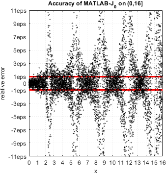
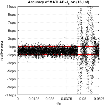
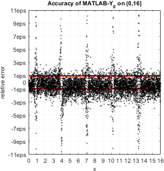
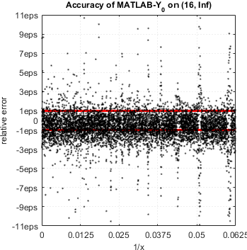
MATLAB’s functions bessely(n,x) and besselj(n,x) are unable to approximate Yn(x) and Jn(x) correctly in neighborhood of its zeros. No single correct digit is produced!
Acknowledgements
As always, this release would not be possible without feedback, support and requests from our dear users. We would like to express sincere gratitude to all of you – thank you all for your care and support!
Special thanks to Brian Gladman for enlightening discussion and for sharing his outstanding work on Chebyshev expansions for special functions. Also to GNU GSL developers for inviting and allowing me to contribute improved approximations for K0(x) and K1(x).

{ 0 comments… add one now }